On Unsupervising Art
tl;dr Is the democratization of art necessarily a bad thing? I don’t believe it is, and in this blog post, I will rant a bit about art and will most likely talk about things I do not fully understand about it, but hey, this is just a blog after all. In the end, I present how I’ve applied Machine Learning algorithms, specifically Unsupervised Learning algorithms such as GANs, $k-$means, and PCA to aid me in an ongoing art project, Latent Fabrics, where I generate huipils.
Intro
Gatekeeping art is, perhaps, one of the things I dislike the most, and one thing I am certainly guilty of doing before (as I am sure most artists have done once in their lives). In a nutshell, this mindset is as follows: nothing is art but what I create and enjoy, and as a corollary, there aren’t quality artists nowadays, except for me and the artists whose work I enjoy. Indeed, I believe this not only applies to artists but almost everyone, as art is an integral part of our lives: form criticizing nowadays music, to not enjoying superhero movies or even looking down at the No. 1 New York Times bestselling book.
Of course, there is a counterpoint to this. Mario Vargas Llosa writes in his book Notes on the Death of Culture:
La literatura light, como el cine light y el arte light, da la impresión cómoda al lector y al espectador de ser culto, revolucionario, moderno y de estar a la vanguardia, con un mínimo esfuerzo intelectual.
In other words, culture and art have been shifting towards a light version, one in which works of art aren’t meant to be thought-provoking or profound, their only goal is to entertain. In turn, this will force artists to never leave the known comfort zone of art that sells. Indeed, this is notorious in music and cinema, where very few writers venture outside what the studios and producers dictate them to do. But is it necessarily a bad thing?
While it is true that this happens, I think that the only difference between art nowadays and classical art is the sheer number of artists and art being created nowadays. Therefore, we are bound to see repetitiveness, the same movie tropes and the same lyrics/beats in music, the same clichés in novels, but this does not mean that you cannot find quality art, you just have to look harder to distinguish it from the noise (of course, this is all still very subjective in my opinion).
Thus, the advent of computers will only aid in further expanding this rift separating what many perceive as good or bad art, even what is and isn’t art. Indeed, nowadays you don’t need a physical canvas or musical instruments, or even spend years studying the human form to create your own runway/clothes. Of course, there have been some controversial works on this subject, perhaps more so how they are reported by the media (which we will explore further on), but the main point is that computers, machines, and software are here to stay, and will most definitely influence every aspect of our lives, art included.
The Future of Art
But what exactly lies in the future of art? It is, of course, hard to tell with certainty, but one can speculate (and most likely be wrong). In the excellent series The Future of Art by Artsy, we are given the perspective of what the future entails for art from different members of the art community. The latest video by Simon Denny delves into the role of technology, and how the curating part of art will most likely be democratized, to much dismay to Mario Vargas Llosa. Carrie Mae Weems sees the positive light of this, as this democratization of art will give voice to those who haven’t been able to participate in something as elite (even elitist) as art. Specifically, marginalized societies as well as marginalized people such as women of color, and she wishes only to be able to see this in the coming years.
Marcel Dzama argues that classical forms of art such as painting and drawing won’t disappear, and I agree: while the newest technologies create exciting, perhaps refreshing works of art, they won’t compete with the old ways, only complement them at most, as many other forms of art have done in the past. Elizabeth Diller brings forth the impact of time in works of art: while some ideas can make sense at the moment they are thought, in architecture, when they are executed, those ideas might not even make sense at all anymore. Indeed, any work of art is fixed in time, but their meaning is constantly evolving, both for the artist as well as the spectator.
Finally, Trevor Paglen agrees with all these points, in that the art of the future won’t be radically different than the art in the present and past. I would add that the thing that would most likely change is the medium of how the artist communicates his or her idea to the public and that medium is being disrupted by computers and computer software. Indeed, now it is possible to add holograms to your expositions, visit a museum with a robot, and even bring works of art to life via virtual reality.
We do, however, have a potentially bleak future in art if we rely too much on plain predictive models. Ashley Rose writes that the landscape of music has been transformed already by Machine Learning, and that music labels have noticed this and are starting to exploit these models. While the first two points mentioned by the author have some merit (one more than the other), it is the latter one that truly worries me. Indeed, it is possible to identify the next musical star, but we have to remember that music, perhaps more so than any other art form, is an ever-changing landscape, and this is most reflected by the popular music genres each decade.
What many executives fail to understand is that Machine Learning models can be used to predict next top hits, but they do so only by using past data. It is not an AI yet, it is merely a predictive model that mimics something that is intelligent, as Prof. Michael Jordan (not to be confused by the basketball player) eloquently puts it (if you don’t have the time, the first couple of minutes are worth it and always in the back of my mind whenever I read a news article about AI). As such, while some trends may be discovered, there will be a lot of bias introduced into the scenes of music production, as if more bias was warranted.
The world of cinema is no stranger to this. The Verge reports that many startups are offering AI producers, skimming through all the available data to obtain the highest-grossing movie possible. Changing actors and seeing how this will affect the movie performance in different markets seems like the best playground for the moviemakers to invest their money in, but to me, this technology is frivolous at best. Since there aren’t many movies produced per year, there are not many historical data to truly create an unbiased predictive model, and so movie producers might end up greenlighting the wrong movies, remaking old classics without need, or even making the wrong castings–perhaps they have adopted these technologies after all. As far as I understand, Machine Learning models are giving them a wrong sense of safety in a world that demands risk for achieving great things, and without the proper risk, we will only have a milquetoast cinema.
Perhaps I should emphasize that, whilst the predictive models are not nigh imperfect, they are of course not useless. From recommending music to recommending the next show to binge-watch, I am open for these tools to enhance the audience experience, not only on these scenarios but on other forms of art as well, such as the plastic arts. However, it must be understood and emphasized that they are a tool only, and it is up to us to both use them wisely and in a meaningful way.
Generative Art
Generative Art warrants another blog post by itself (one I am sure I will make some time in the future) but is a tool that I believe will open the doors to many marginalized communities. As mentioned earlier, Processing lets you generate works of art without the need to have a physical canvas, and that is a huge step in the right direction. However, it is only one step, and I hope there are many more to take in the future.
Generative Design comes hand in hand with generative art, so it is worthwhile to research what is being done and said in this field. Is Generative Design being used at all or just a hype that is bound to die given the high bar that the human mind has for designed objects?
Rain Noe asks the question of where, aesthetically meaning, does generative design belongs to. To him, generative design’s strength lays not in the aesthetic presentation of it, but on the cost and material savings that should happen behind closed curtains, and it’s thse curtains that should be created by an actual human designer. The teams of Autodesk and Airbus seem to agree, as they have designed lattice structures for the partition frames in the Airbus concept plane that is both lightweight and strong, basically saving valuable resources, but still tried to keep this design somewhat hidden from the passengers.

Two rims found in Rain Noe's article, one generated and the other designed by a human. Which would you prefer?
There is nothing wrong with this stance, but I believe that more can be done with Generative Design than simply limiting it to small objects. What if we let a generative algorithm design, with the appropriate constraints, the highways between cities or even a whole city layout? We don’t need to hold the object being designed with our own hands to appreciate its beauty or usefulness, so perhaps we need to set this paradigm loose.
As a final note, I feel that there is frustration in Generative Art and Design on how this field is being reported, especially on the topic of who is the actual artist (the programmer or the machine), or even if it is more appealing than human-generated art. First of all, this is folly in my opinion and only shows a lack of understanding in the area. Second of all, it’s not even an interesting question. However, time will tell whether or not the effort to advance this field was worth it, but my prediction will be that it was.
Machine Learning in Art
Machine Learning has forever changed the panorama of every field it has been introduced to, and art is no exception. Perhaps the ones I enjoy the most, besides image generation, is text and character generation. Projects such as textgenrnn and kanji-rnn show me the power that language has and how we can leverage the potential of Machine Learning to let more and more cultures to express themselves with these tools.

Fake kanji created by kanji-rnn. The model predicts what the next stroke of the *pen* will be, and the results are different as the user advances with their drawing.
While these tools are classical Supervised Learning techniques, I believe a greater potential resides in Unsupervised Learning algorithms. This brings me to the main title of this blog post (a clever wordplay if you will): we need to democratize the techniques found in Unsupervised Learning amongst the art community, nay, amongst the general audience, and quit trying to form clubs where only the elites can reside and mock the uncultured. Otherwise, we are back in the Renaissance, where certainly excellent art was being produced, but only by those who had both the talent and access to the right tools. Hence, we must be open to starting Unsupervising Art.
Perhaps, to illustrate what can be achieved with these techniques, I will tell the tale of one of my latest endeavors, but for that, I will need to delve a bit into a summary of what techniques have been and are being used in the art world.
GANs
We begin our mini summary with Generative Adversarial Networks or GANs, which are perhaps one of the most applied machine learning paradigms to the world of art. We will look at them from the point of view of images, but it can be applied wherever you have a distribution of data that you wish to mimic. The idea is as follows:
- There are two competing neural networks, a generator $G$ and a discriminator $D$, and they are playing a simple zero-sum game.
- The generator must produce images $\mathbf{x} = G(\mathbf{z}; \theta^{(g)})$ and the discriminator will emit a probability $D(\mathbf{x}; \theta^{(d)})$ which will be high (close to $1$) if it believes $\mathbf{x}$ is a real image from our training set or low (close to $0$) if it believes it to be fake.
- We will represent both the generator and discriminator as neural networks, hence the parameters $\theta^{(g)}$ and $\theta^{(d)}$, but we will use either notation interchangeably.
This game will be played until the fake images are indistinguishable from the real ones, or in other words when $D(\mathbf{x}) = 1/2$ always. The fake images will be generated via $G(\mathbf{z})$, where $\mathbf{z}$ will be a random vector drawn from a latent space (a vector space) of representations where any point in said space can be mapped to a realistic-looking image $\mathbf{x}$. It should be noted that this latent space won’t be continuous, unlike one constructed with Variational Autoencoder or VAE.
Since this is a zero-sum game, we define $v (\theta^{(g)}, \theta^{(d)})$ as the reward we give to the discriminator for correctly classifying the fake data from the real one, while we give $-v (\theta^{(g)}, \theta^{(d)})$ as a reward to the generator. At convergence, we will have:
\[G^{\star} = \arg \min_{G} \max_{D} v(G, D)\]Thus, in function of the parameters of the respective neural networks $\theta^{(g)}$ and $\theta^{(d)}$, $v$ should be:
\[v \left(\theta^{(g)}, \theta^{(d)}\right) = \mathbb{E}_{\mathbf{x}\sim p_{\text{data}}(\mathbf{x})} \left[ \log{(D(\mathbf{x}))} \right] + \mathbb{E}_{\mathbf{z}\sim p_{\mathbf{z}}(\mathbf{z})} \left[\log{(1-D(G(\mathbf{z})))} \right]\]This equation can be read as follows: we add both the expected values of the log probability of the discriminator $D$ predicting that the real-world pictures are genuine and the expected values of the log probability of the discriminator $D$ predicting that the images generated by $G$ are not genuine. The reason why we use $\min_{G} \log{(1-D(G(z)))}$ instead of $\max_{G} \log{D(G(z))}$ is to avoid oversaturating the gradients while the neural networks are learning, specifically when $G$ is producing really bad results.
Of course, the question with GANs is always when to stop training the networks: if we train too much, there will be overfitting, and there is no clear rule or criteria on when to stop this learning process. As such, we must babysit the training process and see the results obtained, as it is quite possible to arrive at a local minima and simply start memorizing the data.
Now that this is out of the way, I present my project:
Latent Fabrics
Latent Fabrics began as a project to understand what constitutes a huipil: is there something more profound than the general shape and colors? Are the patterns indicative of something that links the cultures within Mexico and Central America, even if there is no shared history? As such, the first idea I had was to simply build a classifier, born from the constant plagiarism that indigenous textile design suffers from (even outside of the textile world).
Indeed, it is a pressing issue where Machine Learning can (and should) be part of the solution. However, the difficulty in using a classifier is the sheer amount of data needed for it to train and converge, as well as to have each image correctly labeled. As such, this project shifted to try to generate new huipils without the need to label them, and what better candidate for the job than GANs?
For the data, I used Karen Elwell’s Flickr collection (with permission) and for the code implementation, I used Taehoon Jim’s DCGAN in tensorflow. While I started with over 2000 photographs of huipils, many where duplicates and some others could not be used. As such, I ended up with 641 pictures of huipils, specifically from Mexico and Guatemala. Nowadays, Karen’s collection has far more pictures, and I hope to both use the new pictures of huipils, as well as to combine them with other sources such as the Museo Ixchel’s and the Minneapolis Institute of Art (MIA), where I have found on the latter 81 new huipils to use.
The following are the results: after circa 2 days of training the networks on my GeForce 980M, I obtained 221 generated huipils of size $256 \times 256$ pixels and on another separate run of circa 2 days, I obtained 330 generated huipils of size $64 \times 64$ pixels.

The 221 generated huipils of size $256 \times 256$ pixels arranged randomly. Pardon the sheer size of the file.
Of course, the first results I obtained where generating huipils of size $64\times 64$ with the same training time of 2 days on my GPU. If I’m quite frank, I find some of the generated huipils to be quite beautiful. However, I recognize that, due to the size of the training set and the size of the images, this might simply be the first symptoms of overfitting.

The 330 generated huipils of size $64\times 64$ pixels arranged randomly.
All in all, this was the work of weeks, as some hyperparameters were tuned, some pictures were modified to better work for the dataset, and also there were lots of failures. Of course, there are far more huipils that could be generated, but these where the ones that, to my criteria, were most pleasing to the eye. Indeed, this is after all the job of the artist, otherwise, we would let randomness govern us, and the human mind gets easily bored of the random world unless we get to participate in its creation process and curate it.
I was fortunate enough that this piece was accepted at the NeurIPS Workshop on Machine Learning and Creativity from 2018 and shown on its online AI art gallery. For this, I must thank Luba Elliott for her great work in curating the online gallery, as well as for the help provided to me (and all the other artists) during the collection of all the pieces.
Now that we have these generated huipils, what could be the next step? The random arrangement can only get us so far, so why not separate the huipils by likeness to each other? This could be done manually, but, being as lazy as I am, there is another algorithm that can come in handy…
$k$-means Clustering
The final step (thus far) has been to apply the well-known unsupervised learning algorithm $k$-means clustering which partitions a dataset into $k$ distinct, non-overlapping clusters. As with any Unsupervised Learning algorithms, there is no correct answer, so the different results I would obtain would depend largely on how the centroids of each cluster are initiated, any preprocessing done, the pseudo-random numbers used, as well as the implementation of the algorithm itself.
We start by loading some necessary packages:
import numpy as np

from PIL import Image
import glob
import os

import matplotlib.pyplot as plt
import seaborn as sns; sns.set()
Now it’s time to load the generated huipils. These were in a directory with a different name, but we can simply assume its name is images_to_append. We open this directory (I am using Windows 10, hence the \\), and append them to an empty array which we then turn into a NumPy array. Since all the images where PNGs, we used a wildcard *.png. Here is the code:
filepath = os.getcwd() + "\\images_to_append\\"
image_list = []

for filename in glob.glob(filepath+'*.png'):
    im = np.float64(Image.open(filename))
    image_list.append(im)

image_list = np.array(image_list)
num_images = len(image_list)
We check the shape of the image_list array in order to confirm that we have $221$ images of size $256\times 256$, with $3$ color channels:
>>> image_list.shape
(221, 256, 256, 3)
We scale and transform the array since we will be using some dimensionality reduction techniques later on:
from sklearn.preprocessing import StandardScaler

X = StandardScaler().fit_transform(image_list.reshape(num_images, -1))
Note that we have flattened the array via image_list.reshape(num_images, -1), i.e., now the shape will be (221, 196608) (some huge vectors). Now comes the questions of how many clusters to use, i.e., what should the value for $k$ be? There was a simple solution: I want 7 different groups, given that that’s how many frames I was commissioned in delivering. However, it wasn’t the only restriction as I could simply produce more and just deliver 7 frames, or less and then become creative.
A useful guide is to use the Silhouette score, a measure of how similar a data point (in this case, a generated huipil) is to its cluster compared to the others. For this project, I used Scikit-learn’s $k-$means implementation, so we proceed to record, for each value of $k$, what is its respective Silhouette score.
from sklearn.cluster import KMeans

from sklearn.metrics import silhouette_score

sil_score = []

for k in range(2, 20):
    kmeans = KMeans(n_clusters=k, random_state=42).fit(X)
    labels = kmeans.labels_
    sil_score.append(silhouette_score(X, labels, metric='euclidean'))
We plot the resulting array in the vertical axis, with $k$ on the horizontal axis:
plt.figure(figsize=(12,9))
plt.plot([k for k in range(2, 20)], sil_score)
plt.xlabel('Numero de clusters')
plt.ylabel('Score de silueta')
plt.xticks([k for k in range(2, 20)])
plt.show()

Silhouette score for different values of k. While all of them are quite low tbh, $k=7$ does seems promising.
The higher the value, the better, so this seems to confirm that we should use $k=7$. This is what we continue to do and save the labels generated for each huipil (which will be used later on to separate them into distinct files):
kmeans = KMeans(n_clusters=7, random_state=42).fit(X)
labels = kmeans.labels_
We can then print this array, but it’s hard to note anything, to be frank, so we can use Counter to count how many generated huipils are in each cluster/group:
>>> labels
array([2, 3, 0, 1, 0, 2, 1, 2, 4, 4, 3, 5, 2, 0, 1, 6, 0, 0, 3, 1, 6, 0,
       4, 5, 6, 2, 0, 5, 6, 6, 0, 1, 6, 5, 0, 1, 4, 6, 5, 1, 3, 3, 2, 5,
       5, 5, 2, 3, 5, 6, 0, 6, 0, 1, 6, 0, 5, 5, 6, 4, 5, 2, 6, 5, 4, 0,
       5, 4, 4, 0, 4, 5, 6, 4, 6, 1, 4, 0, 6, 2, 2, 6, 4, 2, 2, 5, 6, 5,
       6, 1, 5, 4, 3, 5, 5, 3, 4, 3, 3, 4, 3, 4, 0, 5, 4, 5, 3, 1, 5, 5,
       4, 5, 6, 1, 2, 5, 0, 5, 6, 6, 4, 3, 3, 4, 5, 6, 6, 0, 1, 3, 4, 4,
       0, 4, 5, 5, 2, 4, 6, 4, 3, 0, 6, 3, 4, 2, 3, 3, 6, 6, 1, 0, 1, 5,
       6, 0, 6, 6, 0, 6, 6, 4, 2, 4, 3, 1, 2, 3, 1, 5, 5, 0, 6, 0, 1, 5,
       0, 2, 5, 3, 5, 0, 4, 2, 1, 5, 4, 0, 6, 6, 4, 6, 3, 5, 4, 4, 3, 4,
       6, 5, 4, 6, 5, 4, 1, 6, 2, 4, 5, 6, 6, 5, 4, 5, 6, 5, 2, 1, 0, 5,
       5])
>>> from collections import Counter
>>> Counter(labels)
Counter({0: 29, 1: 21, 2: 21, 3: 24, 4: 38, 5: 46, 6: 42})
This seems quite balanced, so now the question is if we can visualize these groups. The problem is the high dimensionality of the data (i.e., the images), so what we can do is use dimensionality reduction techniques.
PCA
Principal Component Analysis or PCA allows us to summarize the dataset with a smaller number of variables. Indeed, we wish to find some directions, in function of our $196608$ variables, that best summarize the data. As such, it is a great way of data visualization and we use it as follows:
from sklearn.decomposition import PCA

pca = PCA(n_components=100)
projected = pca.fit_transform(X)
We plot the generated huipils using the first two principal components:
plt.figure(figsize=(12,9))
plt.scatter(projected[:, 0], projected[:, 1], c=labels,
            edgecolor='none', alpha=0.9, cmap=plt.cm.get_cmap('Spectral', 7))
plt.xlabel('Componente 1')
plt.ylabel('Componente 2')
plt.colorbar()
plt.show()

Plotting each generated huipil in a reduced dimension space using Principal Components. Note there are natural clusters appearing, but others are more intertwined.
This is a very satisfying result. The question is now whether or not the clusters are intertwined, so we can add a third axis by using the third principal component and we observe the following:

Same as before, but now we add a third dimension.
It seems that the clusters are very well separated. As a final sanity check, we can see how much of the variance of our original dataset is explained as we keep on adding principal components (hence, why we used n_components=100 at the beginning):
plt.figure(figsize=(12,9))
plt.plot([i for i in range(1, 101)], np.cumsum(pca.explained_variance_ratio_))
plt.xlabel('Numero de componentes')
plt.ylabel('Varianza explicada cumulativa')
plt.show()

The explained variance in function of the number of principal components. There is a steep increase at the beginning, so we know that the first components will hold most of the information.
We see that, to explain $70\%$ of the variance, we need $20$ principal components:
>>> next(i for i, v in enumerate(np.cumsum(pca.explained_variance_ratio_)) if v>0.7)
20
This might seem a lot, but remember that we are reducing this from $196608$. This didn’t change our result, so we proceed with separating our generated huipils.
Separating the images
Before moving them with Python, we first create the new directories. If you’re using a Jupyter notebook, you can also run this code by adding a ! at the beginning of the line of code:
>>> FOR /l %x in (0, 1, 6) DO mkdir .\\Project_name\\%x
We create 7 directories/folders with the names of the groups we have created with the $k$-means algorithm. Now we just proceed to copy, into each folder, the corresponding huipil using the labels array:
import shutil

for folders, subfolders, filename in os.walk(filepath):
    i=0
    while i<num_images:
        shutil.copy(filepath+filename[i], os.getcwd()+'\\Project_name\\'+str(labels[i]))
        i+=1
We will then end up with 7 different folders, each containing similar generated huipils (to the algorithm’s criteria). Afterwards, I decided to arrange the images of each folder/label in canvases of $11\times11$ inches, particularly since they were commissioned by my brother. These are the final results, with the names indicating the label of the image (if there were too many images and they didn’t fit, I separated into two):
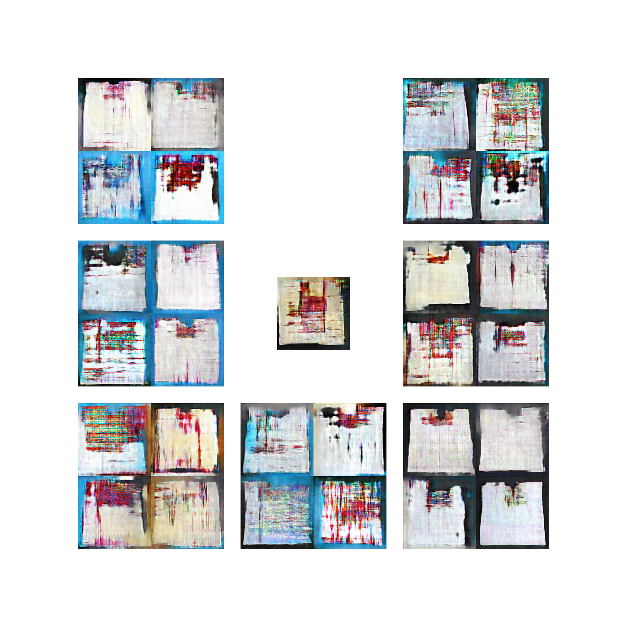
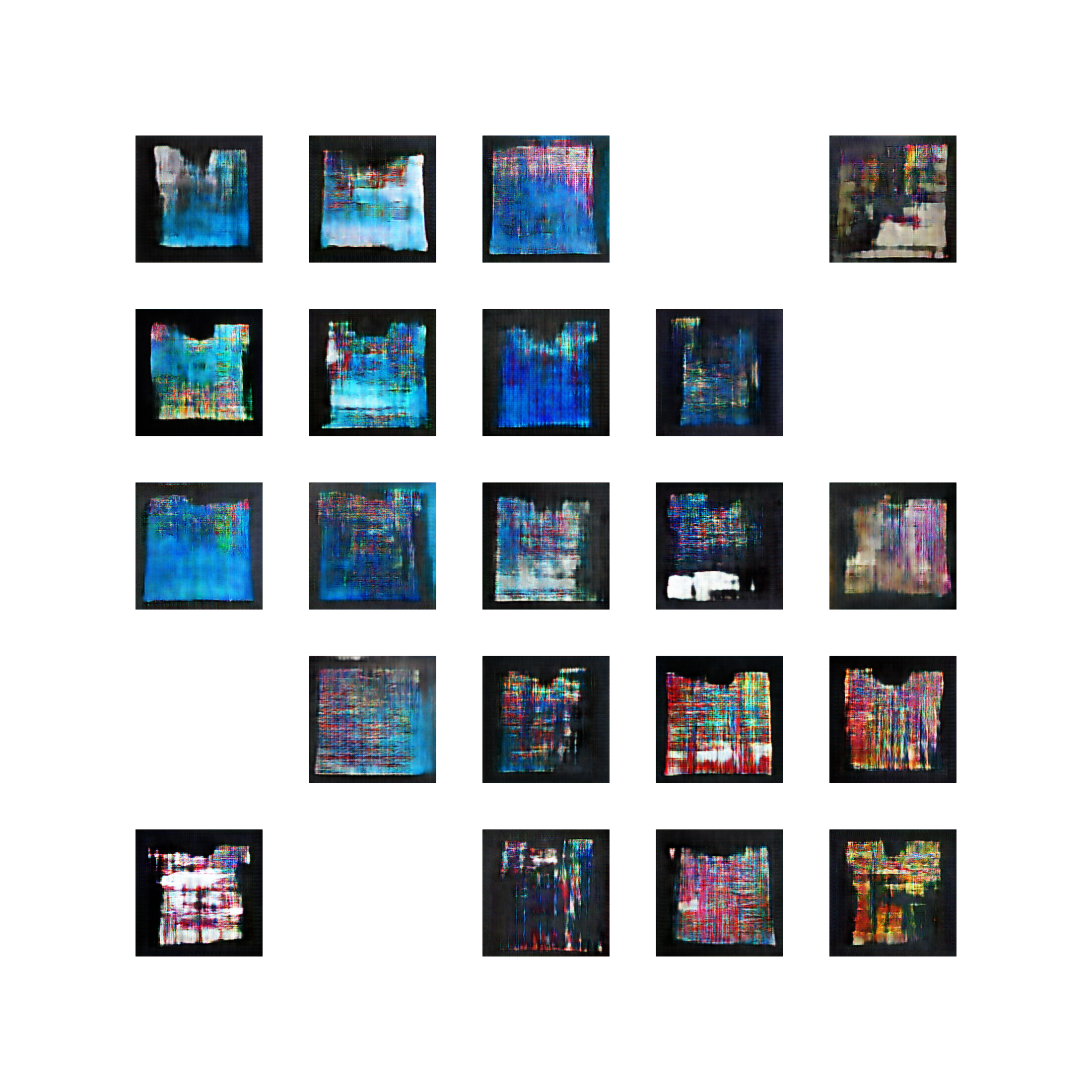


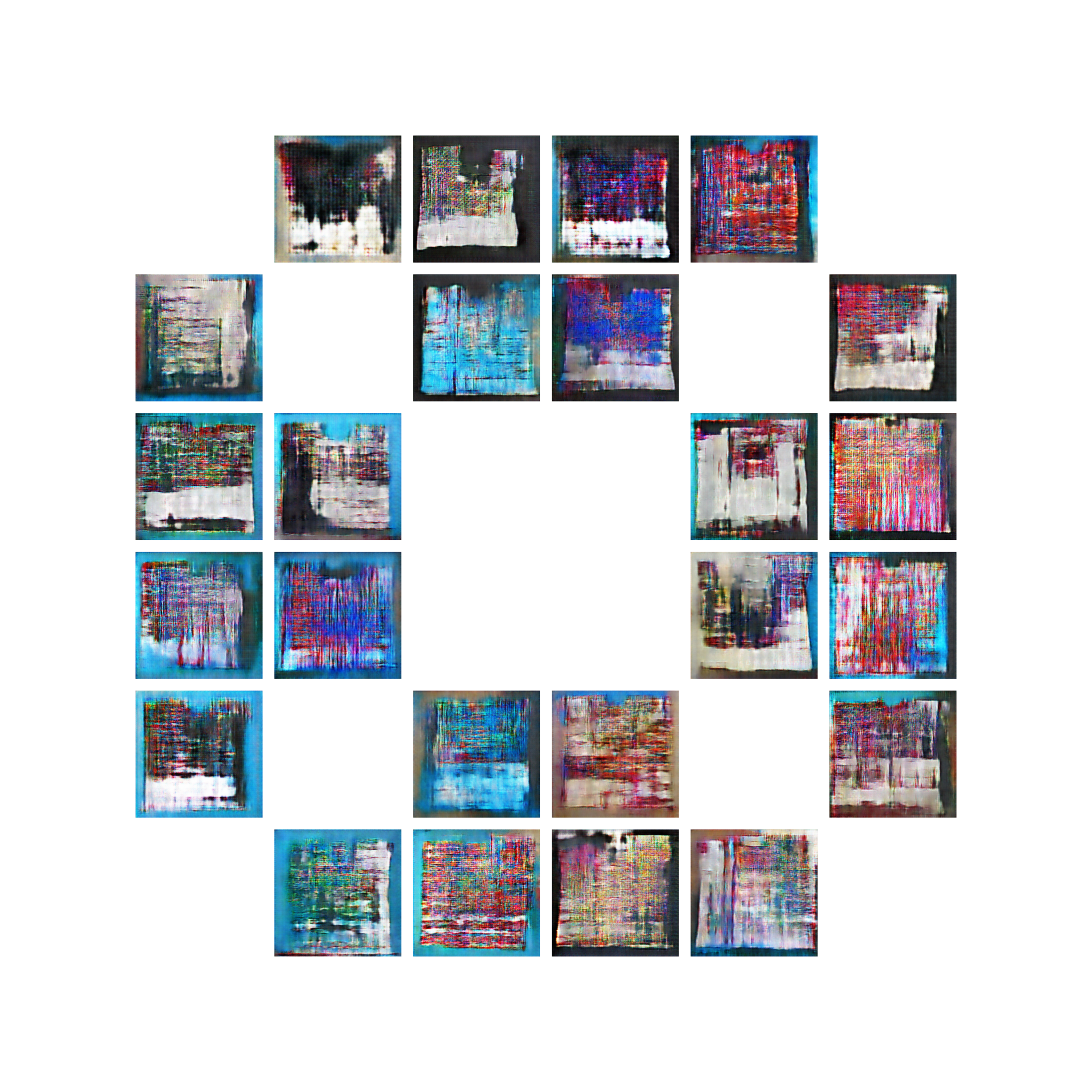
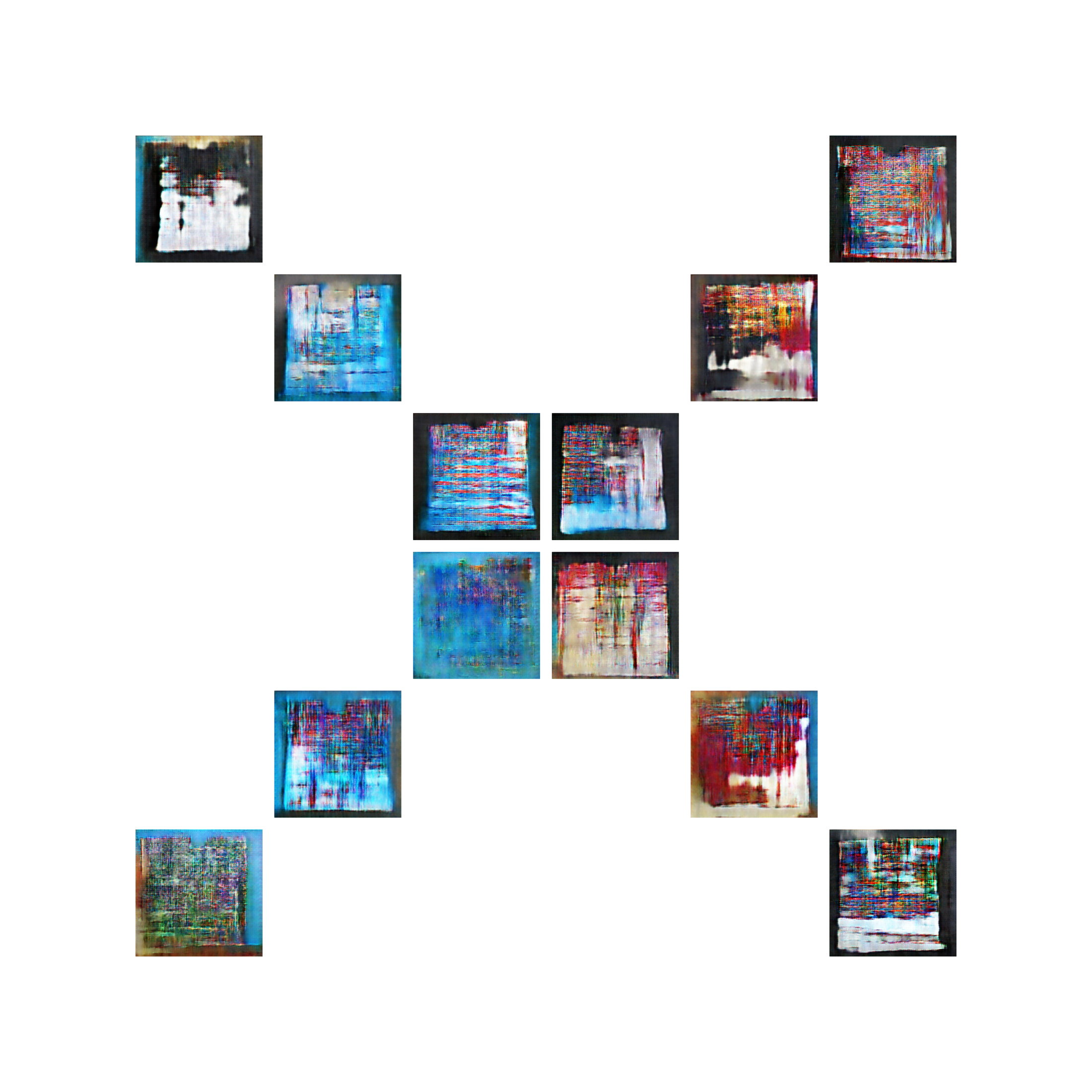

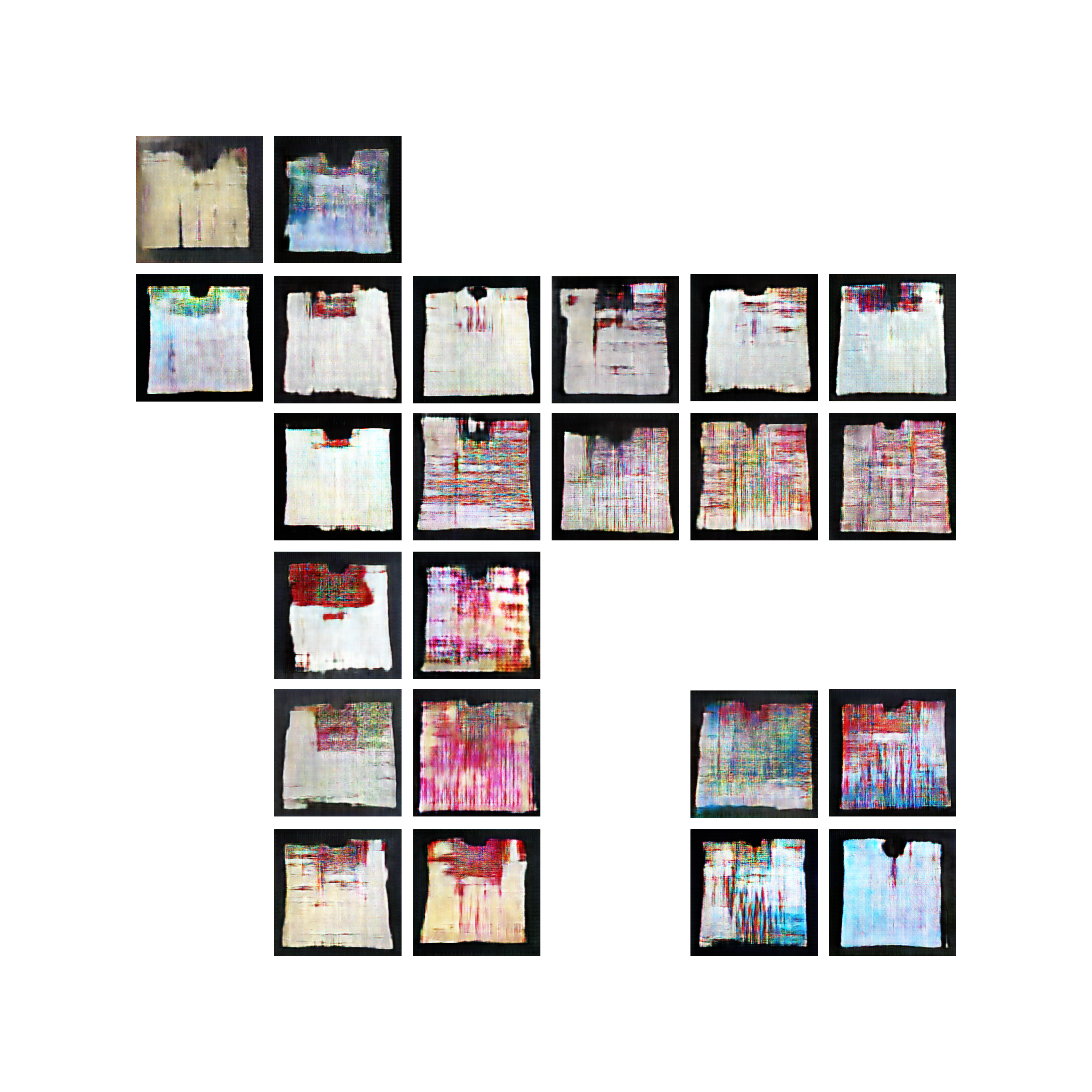


If you use these in any way, please credit me and let me know about it, I won’t get mad!
Next Steps
It is not so obvious what should be the next steps for this project, but I can at least enumerate some. These are, in no particular order:
- Remove the checkerboard artifacts due to the Deconvolution (this can be more easily seen in the $256\times 256$ generated huipils).
- Increase the size of the generated huipils, hopefully up to $1024 \times 1024$, should my hardware allow it. This is because I wish to see more patterns emerge within the generated huipils.
- Train the models for more epochs and with a larger dataset, so basically continue obtaining more images and get better hardware and/or simply train for longer in my laptop. Likewise, clean the original dataset, as I have found both inconsistencies as well as downright bad pictures that slipped my original check.
- Traverse the latent space that weaves all the huipils together (the Latent Fabrics if you will).
- Explore the possibility of combining my work with Processing and add another type of generative art.
- Finally, ponder how to present this work: should digital art remain digital, or does it make sense to bring it to the physical world via another technique, such as actual weaving?
I hope you have enjoyed this blog post. Please leave any comment below!